In a previous article, we installed an HPC cluster on virtual machines. Let’s write a program that uses the HPC cluster to compute an approximate value of pi. We will see how to distribute a task on multiple compute nodes, and how to efficiently aggregate all results on the master node using MPI in C++.
Computing pi using Monte Carlo integration
To compute pi, we use a Monte Carlo integration technique. The idea is to repeatedly sample the domain of the function we want to integrate and count how many samples land in the function versus outside the function. For pi, we want to integrate a quarter of the unit disk, whose area is pi/4. Although there are more elaborate Monte Carlo techniques, we stick with the basic just to get started.
Here is the algorithm:
- We sample N points randomly on the unit square a. We count the number M of random samples that land into the unit disk
- Pi is approximately equal to 4M/N
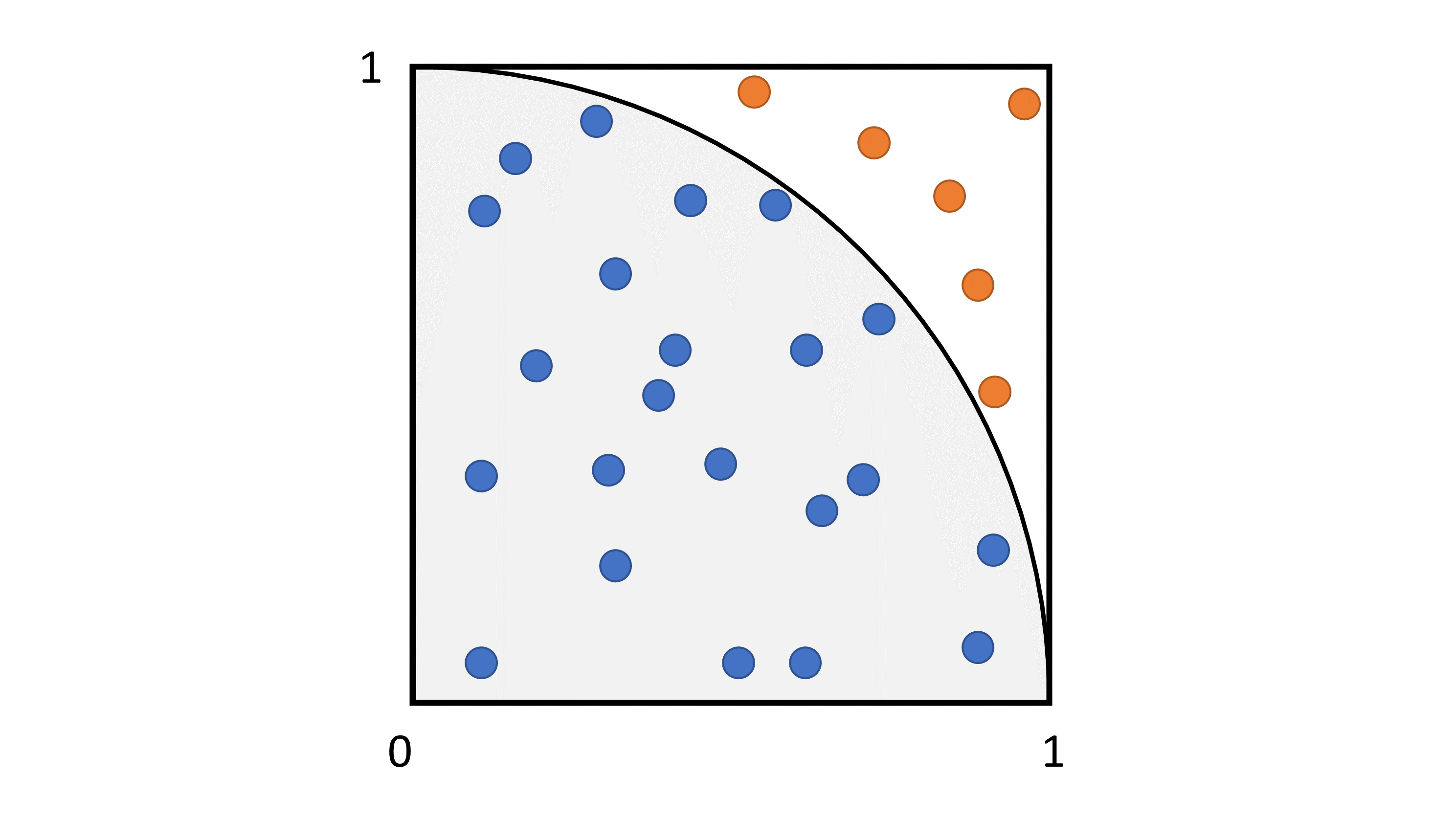
Following is a diagram to get a better understanding of how random samples are used to compute pi.
 In this figure, the square represents the unit square, the circle represents a quarter of the unit disk. Dots represent all the random samples among which blue dots are in the unit disk, and orange dots are outside the unit disk but inside the unit square. In this case, with 22 samples in the disk and 28 total samples, the approximation of pi is
 pi=4*22/28=3.1428...
Parallelizing computations
The simplest approach to parallelize the computation of pi with Monte Carlo is to split the random generation and the counting of samples on multiple processes. Each node of our cluster will draw n random points in the unit square, and check whether they are in the unit disk or not. Note that when parallelizing this algorithm, there is a fine detail that we absolutely need to pay attention to. The random number generators need to be initialized with a different seed on each node. Otherwise, all nodes will generate the exact same sequence of random samples. Not only it defeats the purpose of parallelizing, but also the computation will be biased, and we will most likely not get the correct approximation of pi.
// Initialize the random number generator, make sure the seed is different on each node
// By using the the formula s = a*x + b*y, we minimize the probability of collisions for the seeds
unsigned seed = std::chrono::system_clock::now().time_since_epoch().count();
std::mt19937_64 random_generator(449251 * seed + 26722 * world_rank);
Now here is an interesting question: how are the individual samples added up together to form the final result? We will see that there are multiple approaches, some of which are more efficient than others.
Naïve implementation with MPI_Send and MPI_Recv
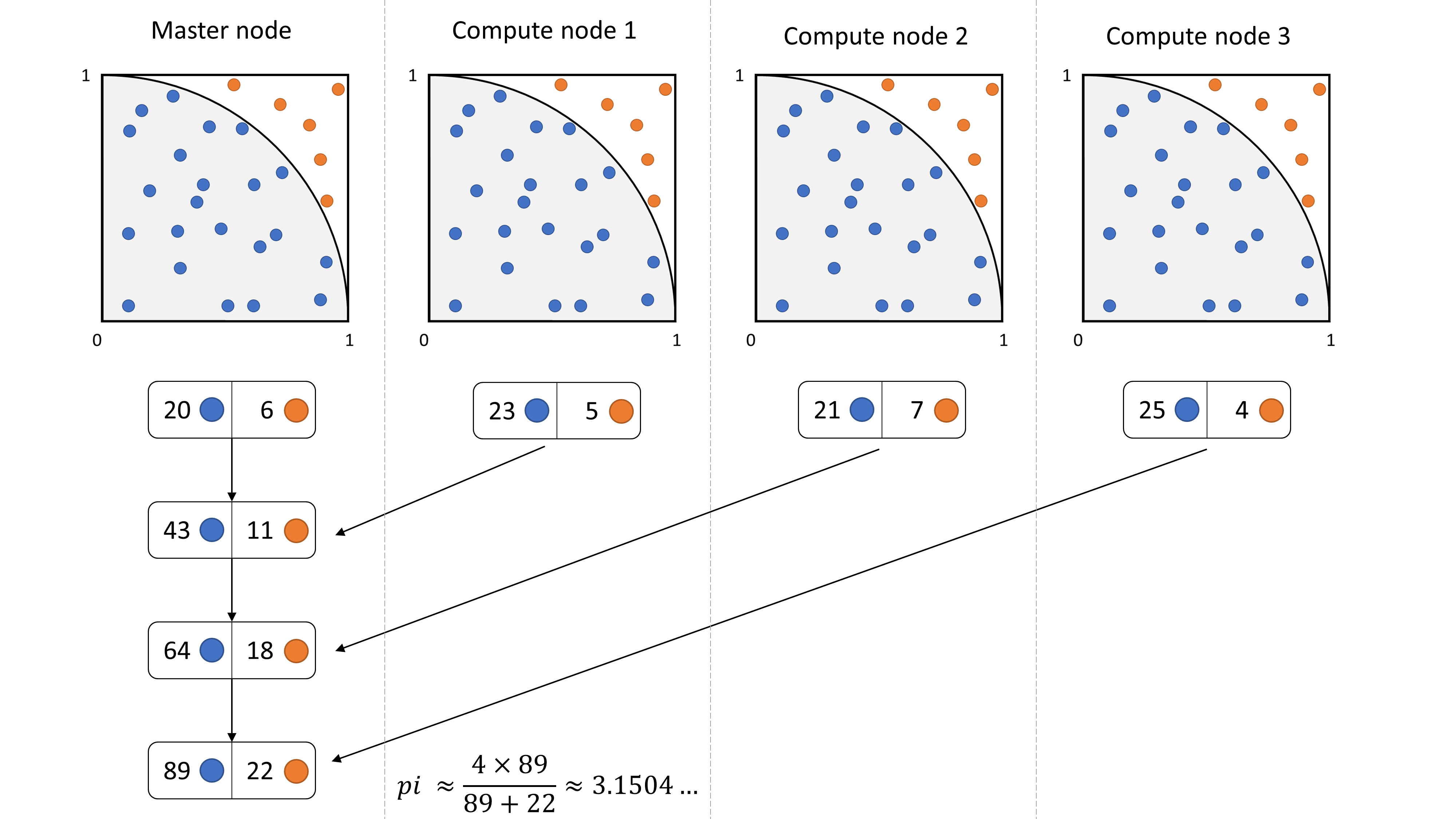
The most straightforward method is to send all partial results to the master node when computations are done.
// Compute values locally on each processor
auto [circle_points, square_points] = estimate_pi(random_generator, n);
// Naive reduce implementation, implemented using MPI_Send and MPI_Recv
int64_t global_circle_points = circle_points;
int64_t global_square_points = square_points;
if (world_rank == 0)
{
    // The master node receives from all other nodes
    for (int source = 1; source < world_size; source++)
    {
        MPI_Status status;
        MPI_Recv(&circle_points, 1, MPI_LONG_LONG, source, 0, MPI_COMM_WORLD, &status);
        MPI_Recv(&square_points, 1, MPI_LONG_LONG, source, 0, MPI_COMM_WORLD, &status);
        global_circle_points += circle_points;
        global_square_points += square_points;
    }
}
else
{
    // All nodes send their result to the master
    MPI_Send(&circle_points, 1, MPI_LONG_LONG, 0, 0, MPI_COMM_WORLD);
    MPI_Send(&square_points, 1, MPI_LONG_LONG, 0, 0, MPI_COMM_WORLD);
}
Here is a diagram showing what is happening with 4 processes:

Efficient implementation with MPI_Reduce
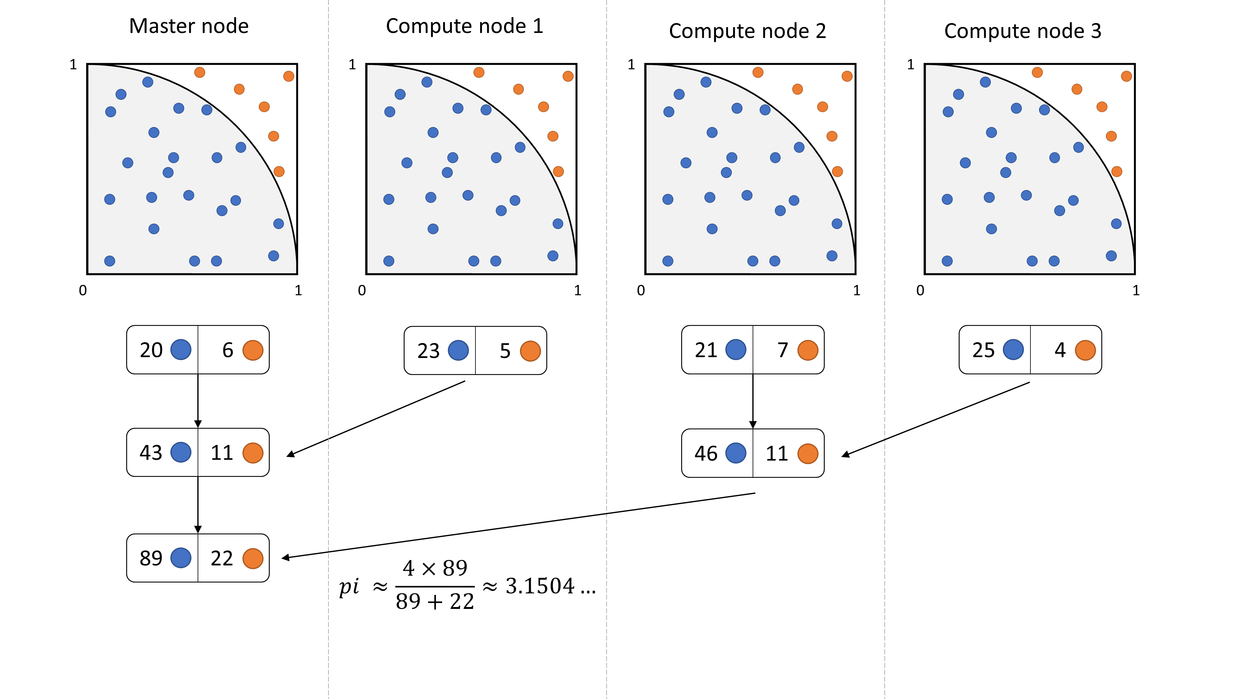
A more interesting method is to use a tree structured communication to aggregate the results to the master node. In fact, one drawback of the naïve approach is that almost all the compute nodes are idle while the master node is aggregating results. By using a tree structured communication pattern, we maximize the utilization of compute node, and therefore we decrease the total number of communication stages from o(n) to o(log n). This can be a huge savings.
// Compute values locally on each processor
auto [circle_points, square_points] = estimate_pi(random_generator, n);
// Efficient reduce implementation, implemented using MPI_Reduce
MPI_Reduce(&circle_points, &global_circle_points, 1, MPI_LONG_LONG, MPI_SUM, 0, MPI_COMM_WORLD);
MPI_Reduce(&square_points, &global_square_points, 1, MPI_LONG_LONG, MPI_SUM, 0, MPI_COMM_WORLD);
In this implementation we use the MPI_Reduce function that is part of the MPI standard. The purpose of this function to make reductions efficiently by using a tree reduction. Furthermore, on supercomputers, it is possible to have a custom implementation of this routine that is more efficient because it works with the specific network architecture in mind.
Here is a diagram showing what is happening with 4 processes:

Performance comparison
I ran my code on one of the university supercomputers: Halstead. It has nodes with 20 cores and InfiniBand interconnection. I ran the naïve as well as the efficient implementations on 1 and 5 nodes to see if there are any benefits in using the efficient implementation. Following is a table with timings:
| Naïve on 20 cores | Efficient on 20 cores | Naïve on 100 cores | Efficient on 100 cores | |
|---|---|---|---|---|
| Run 1 | 0.0848 s | 0.0350 s | 0.2444 s | 0.1872 s |
| Run 2 | 0.0622 s | 0.0481 s | 0.2305 s | 0.1908 s |
| Run 3 | 0.0624 s | 0.0653 s | 0.2507 s | 0.1773 s |
| Run 4 | 0.0624 s | 0.0426 s | 0.2313 s | 0.1127 s |
| Run 5 | 0.0644 s | 0.0424 s | 0.2507 s | 0.0737 s |
| Mean | 0.0672 s | 0.0467 s | 0.2415 s | 0.1484 s |
| Std | 0.0099 s | 0.0114 s | 0.0100 s | 0.0524 s |
As we can see, in both cases the efficient implementation is significantly faster than the naïve implementation.
Computing an approximation of pi
Now that we have seen an interesting fact about programming with MPI, one question remains. Is our implementation any good for approximating the value of pi? Well unfortunately, the answer is no. When running the code with 1 billion samples, the result is consistently precise up to 3 digits, and it takes a couple of seconds on my laptop. I even ran it on one of the university supercomputers with 10 billion samples, I got the following result in about 5.5 seconds on 100 cores: pi = 3.14161. Although this code is terrible for estimating PI, it is nevertheless a good example on how to use MPI for distributing a simple computation on many nodes and aggregating the results. Although this approach for computing pi is a waste of time and resources, it is an interesting baseline, and we will see better approaches in the future.
Full code
#include <iostream>
#include <cstdint>
#include <tuple>
#include <random>
#include <chrono>

#include <mpi.h>

// Activate this define to test the naive implementation of the reduce operation
// #define NAIVE_REDUCE

template<class Generator>
std::tuple<int64_t, int64_t> estimate_pi(Generator& random_generator, int n)
{
    // Number of total random points
    const int64_t square_points = n;
    // Number of points in the circle
    int64_t circle_points = 0;

    std::uniform_real_distribution<double> distribution(0.0, 1.0);

    for (int i = 0; i < n; i++)
    {
        const double x = distribution(random_generator);
        const double y = distribution(random_generator);

        const double dist_sq = x*x + y*y;

        if (dist_sq <= 1.0)
        {
            circle_points++;
        }
    }

    return { circle_points, square_points };
}

int main(int argc, char** argv)
{
    MPI_Init(NULL, NULL);

    int world_size, world_rank;
    MPI_Comm_size(MPI_COMM_WORLD, &world_size);
    MPI_Comm_rank(MPI_COMM_WORLD, &world_rank);

    // Total number of random samples
    const int total_n = 1000000000;
    // Number of random samples per task
    const int n = total_n / world_size;

    // Initialize the random number generator, make sure the seed is different on each node
    // By using the the formula s = a*x + b*y, we minimize the probability of collisions for the seeds
    unsigned seed = std::chrono::system_clock::now().time_since_epoch().count();
    std::mt19937_64 random_generator(449251 * seed + 26722 * world_rank);

    const double start_time = MPI_Wtime();

    // Compute values locally on each processor
    auto [circle_points, square_points] = estimate_pi(random_generator, n);

    // Reduce (sum) from all nodes to the root node
    int64_t global_circle_points, global_square_points;

#ifdef NAIVE_REDUCE
    // Naive reduce implementation, implemented using MPI_Send and MPI_Recv
    global_circle_points = circle_points;
    global_square_points = square_points;
    if (world_rank == 0)
    {
        // The master node receives from all other nodes
        for (int source = 1; source < world_size; source++)
        {
            MPI_Status status;
            MPI_Recv(&circle_points, 1, MPI_LONG_LONG, source, 0, MPI_COMM_WORLD, &status);
            MPI_Recv(&square_points, 1, MPI_LONG_LONG, source, 0, MPI_COMM_WORLD, &status);
            global_circle_points += circle_points;
            global_square_points += square_points;
        }
    }
    else
    {
        // All nodes send their result to the master
        MPI_Send(&circle_points, 1, MPI_LONG_LONG, 0, 0, MPI_COMM_WORLD);
        MPI_Send(&square_points, 1, MPI_LONG_LONG, 0, 0, MPI_COMM_WORLD);
    }
#else
    // Efficient reduce implementation, implemented using MPI_Reduce
    MPI_Reduce(&circle_points, &global_circle_points, 1, MPI_LONG_LONG, MPI_SUM, 0, MPI_COMM_WORLD);
    MPI_Reduce(&square_points, &global_square_points, 1, MPI_LONG_LONG, MPI_SUM, 0, MPI_COMM_WORLD);
#endif

    const double end_time = MPI_Wtime();

    // Only the master node computes the final result
    if (world_rank == 0)
    {
        const double pi = static_cast<double>(4 * global_circle_points) / global_square_points;
        std::cout << "pi = " << pi << std::endl;
        std::cout << "Calculated on " << world_size << " processors in "
                  << end_time - start_time << " s" << std::endl;
    }

    MPI_Finalize();

    return 0;
}
References
- Chapter 4 of Parallel programming with MPI from Peter S. Pacheco
- Estimating the value of Pi using Monte Carlo on GeeksForGeeks